Super Savers are a special breed.

They are not concerned about keeping up impressions; they exist outside the mainstream of seductive consumerism.

Call it a mindset, call it walking a different path; perhaps it’s an offbeat childhood money script. Whatever it is, those who fall into this category or save 20% or more of their income on a consistent basis are members of an elite group who strive for early financial independence.

Speaking of independence: At RIA we believe households should maintain 3-6 months of living expenses in a savings account for emergencies like car and house repairs.  They should also maintain an additional 6 months of living expenses as a “Financial Vulnerability Cushion,”  whereby cash is set aside for the big, life-changing stuff like extended job loss especially as we believe the economy is in a late-stage expansionary cycle. Job security isn’t what it used to be; best to think ahead.

In 2018, TD Ameritrade in conjunction with Harris Poll, completed a survey among 1,503 U.S. adults 45 and older to understand the habits that set Super Savers apart from the pack. The results are not surprising. However, they do validate habits all of us should adopt regardless of age.

Like a physical exercise regimen, shifting into Super Saver mode takes small, consistent efforts that build on each other.

So, what lessons can be learned from this elite breed?

First, on average, Super Savers sock away 29% of their income compared to non-super savers. 

Super Savers place saving and investing over housing and household expenses.

Keep in mind, the Personal Saving Rate as of December 2019 according to the Federal Reserve Bank of St. Louis was a paltry 7.6%.  How does this group manage to accomplish such an arduous task? They abhor the thought of being house poor. They focus attention on the reduction of spending on the big stuff, or the fixed costs that make a huge impact to cash flow. Candidly, they’re not concerned about cutting out lattes as a viable strategy to save money. Super Savers spend 14% on housing, 16% on essential household expenses compared to non-supers who spend 23% and 21%, respectively. Any way you cut it, that’s impressive!

Perhaps it’s because Super Savers think backwards, always with a financially beneficial endgame in mind. There is great importance placed on financial security, peace of mind and freedom to do what they want at a younger age. They consider the cumulative impact of monthly payments on their bottom line, which is not common nature for the masses.  They internalize the opportunity cost of every large or recurring expenditure.

Super Savers weigh the outcome of every significant purchase, especially discretionary items, which invariably increases their hesitancy to spend. This manner of thought provides breathing room to deliberate less expensive alternatives and thoroughly investigate the pros and cons of their decisions.

Tip for the Super Saver in training: Sever the mental connection between monthly payments and affordability. How? First, calculate the interest cost of a purchase. For example, let’s say you’re looking to purchase an automobile. First, never go further than 36 months if you must make payments. Why? Because longer loan terms like 48 to 72 months is a payment mentality that will undoubtedly increase interest costs.

For example, let’s say an auto purchase is financed for $23,000. At 3.49% for 36 months, the payment is roughly $674 with total loan interest of $1,258. For 72 months, naturally there’s a lower monthly obligation – $354. However, total loan interest amounts to $2,525.

A Super Saver’s consideration would be on the interest incurred over the life of a loan, not the affordability of monthly payments. An important difference between this manner of thinking and most, is to meet a lifestyle, it’s common for households to go for the lowest monthly payment with little regard to overall interest paid. Super savers will either consider a less expensive option or adjust household budgets to meet higher payments just to pay less interest in the long run.

Second, Super Savers live enriching lives; they don’t deprive themselves.

Members of the super crowd don’t live small lives -a big misnomer. I think people are quick to spread this narrative to ease personal guilt or envy. Certainly, a fiscal discomfort mindset is part of who they are when they believe personal financial boundaries are breached. However, the TD Ameritrade survey shows that both super and non-super savers spend the same 7% of their income on vacations!

Third, starting early is key for Super Savers.

Per the study, more than half of Super Savers started investing by age 30 (54%).  I’m not a fan of personal finance dogma. Many of the stale tenets preached by the brokerage industry are part of a self-serving agenda to direct retail investor cash into cookie-cutter asset allocation portfolios; all to appease shareholders.

However, one rule I’m happily a complete sucker for is Pay Yourself First. It’s not just a good one. It’s the core, the very foundation, of every strong financial discipline. Why? Paying yourself first, whereby dollars are directed to savings or investments before anything else, reflects a commitment to delayed gratification. An honorable trait that allows the mental breathing room to avoid impulse buys, raise the bar on savings rates and minimize the addition of debt.

Per Ilene Strauss Cohen, Ph.D. for Psychology Today, people who learn how to manage their need to be satisfied in the moment thrive more in their careers, relationships, health and finances when compared to those who immediately give in to gratification. Again, the root of Pay Yourself First is delayed gratification; the concept goes back further than some of the concepts the financial industry has distorted just to part you from your money.

Fourth, Super Savers embrace the simple stuff.

When it comes to financial decisions, basics work. For example, Super Savers avoid high-interest debt (65% vs. 56% for non-super savers),  stick to a budget (60% vs. 49%), invest in the market (58% vs. 34%) and max out retirement savings (55% vs. 30%).

Listen, these steps aren’t rocket science; they’re basic financial literacy.

For example, I’ve been ‘pencil & paper’ budgeting since I began my Daily News Brooklyn paper route at age 11. Budgeting over time fosters an awareness of household cash flow.  Try micro-budgeting for a few months. It will help you intimately engage with  personal spending trends.

Micro-budgets are designed to increase awareness through simplicity.

Yes, they’re a bit time-consuming, occasionally monotonous; however the goal is worth it – to uncover weaknesses and strengths in your strategy and build a sensitivity to household cash-flow activities. My favorite old-school book for budgeting comes from the Dome companies. For a modest investment of $6.50, a Dome Budget Book is one of the best deals on the market.

Last, Super Savers believe in diversified streams of income and accounts!

44% of Super Savers prefer to bolster already impressive savings rates by funding diversified sources of income, compared to only 36% of their non-super brethren. In addition, Super Savers are especially inclined to lean into Roth IRAs compared to non-super savers. It is rewarding to discover how the best of savers seek various income streams to build their top-line.  They are also tremendous believers in Roth IRAs. The reason I’m glad is this information further validates why our advisors and financial planning team members have passionately communicated the importance of the diversification of accounts for several years.

Super Savers build the following income streams outside of employment income – Dividends, investment real estate, annuities (yes, annuities – 21% vs. 14% for non-super savers), and business ownership (14% compared to 8%).

Their retirement accounts are diversified; over 53% of Super Savers embrace Roth options (53% compared to 29%). A great number of Super Savers fund Health Savings Accounts and strive to defer distributions until retirement when healthcare costs are expected to increase.

Why diversification of accounts?

Imagine never being able to switch lanes as you head closer to the destination called retirement. Consider how suffocating it would be to never be able to navigate away from a single-lane road where all distributions are taxed as ordinary income. There lies the dysfunctional concept that Super Savers are onto – They do not believe every investment dollar should be directed to pre-tax retirement accounts.

Congratulations -With the full support of the financial services industry you’ve created a personal tax time bomb!

As you assess the terrain for future distributions, tax diversification should be a priority.  Envision a retirement paycheck that’s a blend of ordinary, tax-free and capital gain income (generally taxed at lower rates than ordinary income). The goal is to gain the ability to customize your withdrawal strategy to minimize tax drag on distributions throughout retirement. Super Savers have figured this out. Regardless of your savings habits, you should too.

Many studies show that super savers are independent thinkers. Working to create and maintain a lifestyle that rivals their neighbors is anathema to them.

Now, as a majority of Americans are utilizing debt to maintain living standards, Super Savers set themselves apart as a badge of courage. No doubt this group is unique and are way ahead at crafting a secure, enjoyable retirement. and financial flexibility. Whatever steps taken to join their ranks will serve and empower you with choices that those with overwhelming debt cannot consider.

And speaking of badges: Did you know Amazon sells Merit badges for adulting? It’s true. I believe they need to add a “I’M A SUPER SAVER” badge to the collection.

If you’d like to read the complete T.D. Ameritrade survey, click here.

When I was growing up, my father used to tell me I should “never take advice from anyone who hasn’t succeeded at what they are advising.” 

The most truth of that statement is found in the financial press, which consists mostly of people writing articles and giving advice on topics where they have little experience, and in general, have achieved no success.

The best example came last week in an email quoting:

“You recently suggested that you took profits from your portfolios; however, I read an article saying retirees shouldn’t change their strategies. ‘If you’ve got a thoughtful financial plan and a diversified investment portfolio, the general rule is to leave everything alone.'” 

This seems to be an entirely different approach to what you are suggesting. Also, since corrections can’t be predicted, it seems to make sense.” 

One of the biggest reasons why investors consistently underperform over the long-term is due to flawed investment advice.

Let me explain.

Corrections & Bear Markets Matter

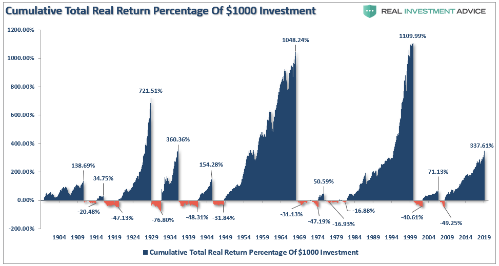
It certainly seems logical, by looking the 120-year chart of the market, that one should just stay invested regardless of what happens. Eventually, as the financial media often suggests, the markets always get back to even. One such chart is the percentage gain/loss chart over the long-term, as shown below.

This is one of the most deceptive charts an advisor can show a client, particularly one that is close to, or worse in, retirement.

The reality is that you DIED long before ever achieving that 8% annualized long-term return you were promised. Secondly, math is a cruel teacher.

Visually, percentage drawdowns seem to be inconsequential relative to the massive percentage gains that preceded them. That is, until you convert percentages into points and reveal an uglier truth.

It is important to remember that a 100% gain on a $1000 investment, followed by a 50% loss, does not leave you with $1500. A 50% loss wipes out the previous 100% gain, leaving you with a 0% net return.

For retirees, this is a critically important point.

In 2000, the average “baby boomer” was around 45-years of age. The “dot.com” crash was painful, but with 20-years to go before retirement, there was time to recover. In 2010, following the financial crisis, the time to retirement for the oldest boomers was depleted, and the average boomer only had 10-years to recover. During both of these previous periods, portfolios were still in accumulation mode. However, today, only the youngest tranche of “boomers,” have the luxury of “time” to work through the next major market reversion. (This also explains why the share of workers over the age of 65 is at historical highs.) 

With the majority of “boomers” now faced with the implications of a transition into the distribution phase of the investment cycle, such has important ramifications during market declines. The following example shows a $1 million portfolio with, and without, an annualized 4% withdrawal rate. (We are going into much deeper analysis on this in a moment.)

While a 10% decline in the market will reduce a portfolio from $1 million to $900,000, when combined with an assumed monthly withdrawal rate, the portfolio value is reduced by almost 14%. This is the result of taking distributions during a period of declining market values. Importantly, while it ONLY requires a non-withdrawal portfolio an 11.1% return to break even, it requires nearly a 20% return for a portfolio in the distribution phase to attain the same level.

Impairments to capital are the biggest challenges facing pre- and post-retirees currently. 

This is an important distinction. Most articles written about retirees, or those ready to retire, is an unrealized assumption of an indefinite timeline.

While the market may not be different than it has been in the past. YOU ARE!

Starting Valuations Matter

As I have discussed previously, without understanding the importance of starting valuations on your investment returns, you can’t understand the impact the market will have on psychology, and investor behavior.

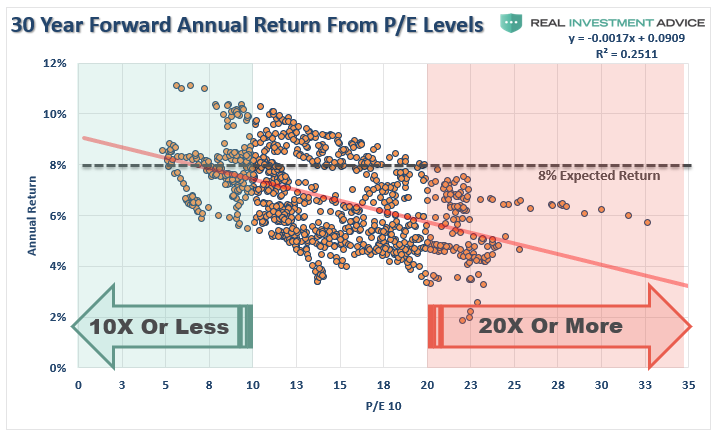
Over any 30-year period, beginning valuation levels have a tremendous impact on future returns.

As valuations rise, future rates of annualized returns fall. This should not be a surprise as simple logic states that if you overpay for an asset today, the future returns must, and will, be lower.

This is far less than the 8-10% rates of return currently promised by the Wall Street community. It is also why starting valuations are critical for individuals to understand when planning for both the accumulation and distribution, phases of the investment life-cycle.

Let’s elaborate on our example above.

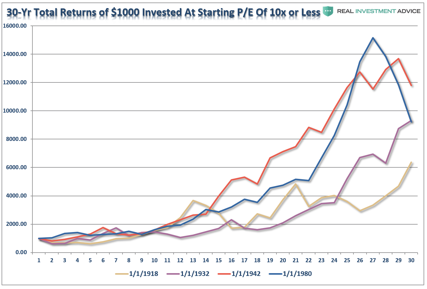
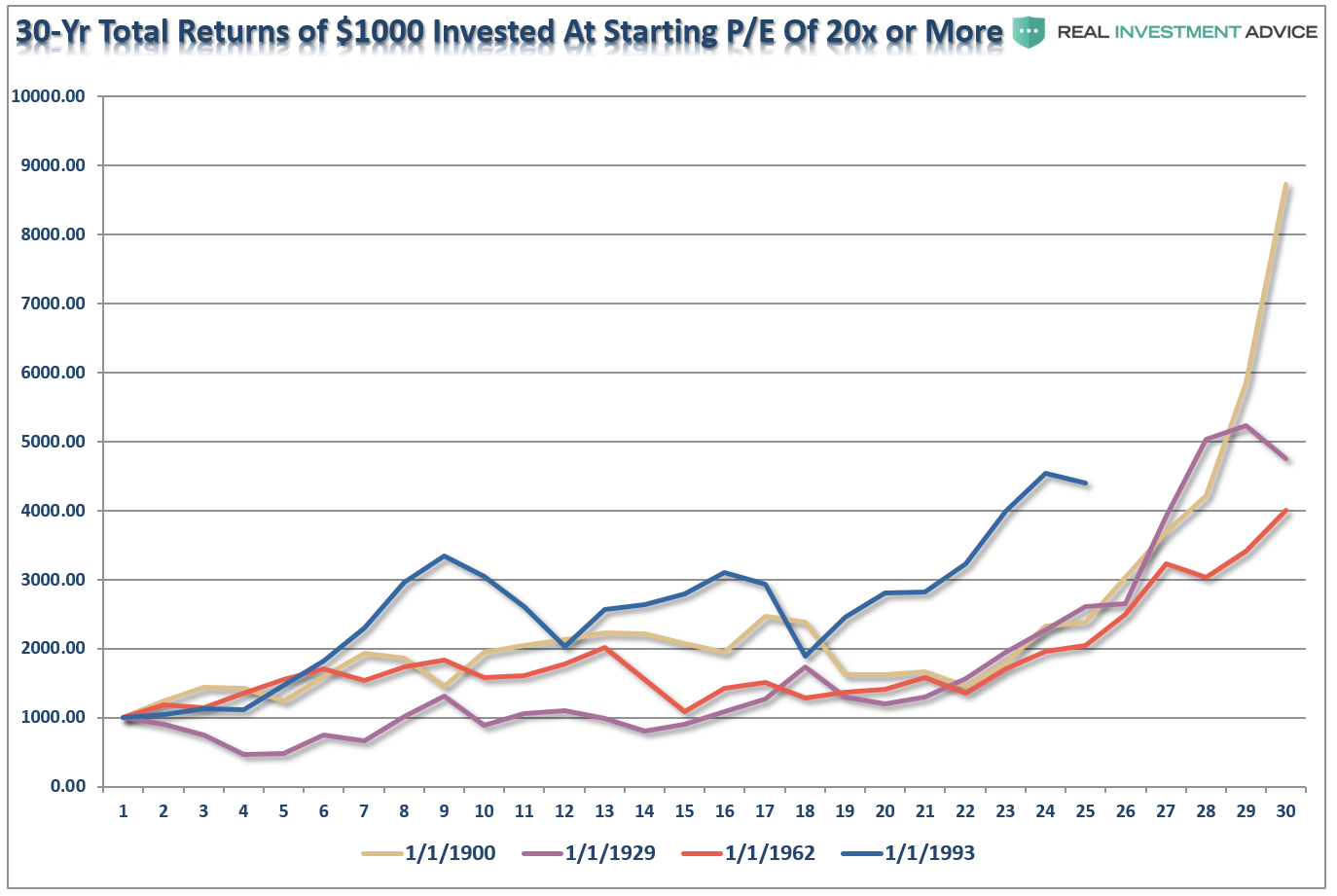
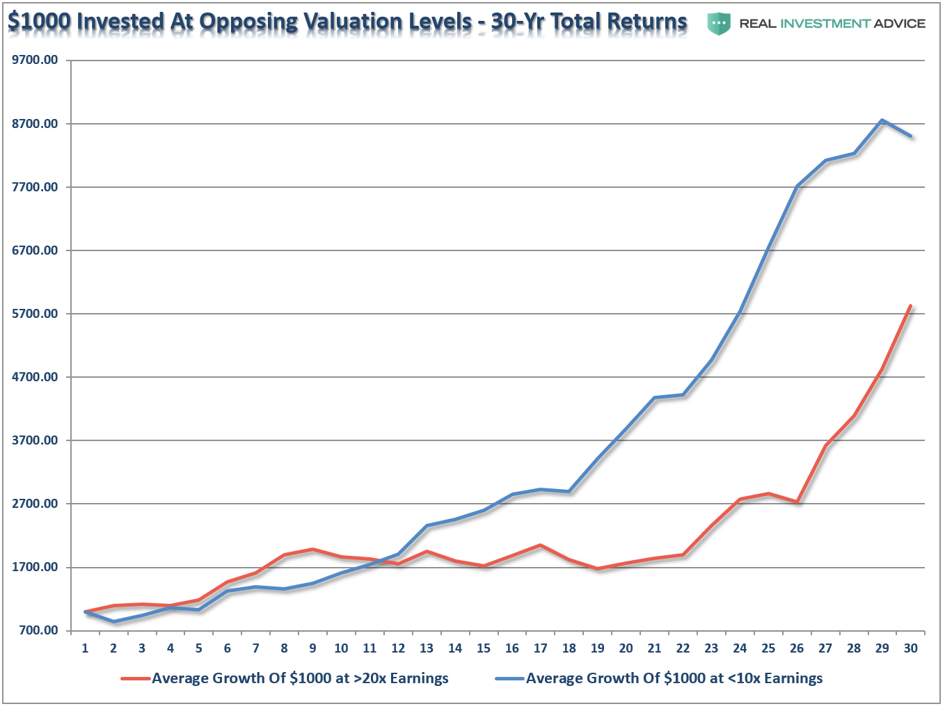
We know that markets go up and down over time, therefore when advisors use “average” or “annualized” rates of return, results often deviate far from reality. However, we do know from historical analysis that valuations drive forward returns, so using historical data, we calculated the 4-periods where starting valuations were either above 20x earnings, or below 10x earnings. We then ran a $1000 investment going forward for 30-years on a total-return, inflation-adjusted, basis. 

The results were not surprising.

At 10x earnings, the worst performing period started in 1918 and only saw $1000 grow to a bit more than $6000. The best performing period was actually not the screaming bull market that started in 1980 because the last 10-years of that particular cycle caught the “dot.com” crash. It was the post-WWII bull market that ran from 1942 through 1972 that was the winner. Of course, the crash of 1974, just two years later, extracted a good bit of those returns.

Conversely, at 20x earnings, the best performing period started in 1900, which caught the rise of the market to its peak in 1929. Unfortunately, the next 4-years wiped out roughly 85% of those gains. However, outside of that one period, all of the other periods fared worse than investing at lower valuations. (Note: 1993 is still currently running as its 30-year period will end in 2023.)

The point to be made here is simple and was precisely summed up by Warren Buffett:

“Price is what you pay. Value is what you get.” 

To create our variable return assumption model, we averaged each of the 4-periods above into a single total return, inflation-adjusted, index. We could then see the impact of $1000 invested in the markets at both valuations BELOW 10x trailing earnings, and ABOVE 20x. Investing at 10x earnings yields substantially better results.

Starting Valuations Are Critical To Withdrawal Rates

With a more realistic return model, the impact of investing during periods of high valuations becomes more evident, particularly during the withdrawal phase of retirement.

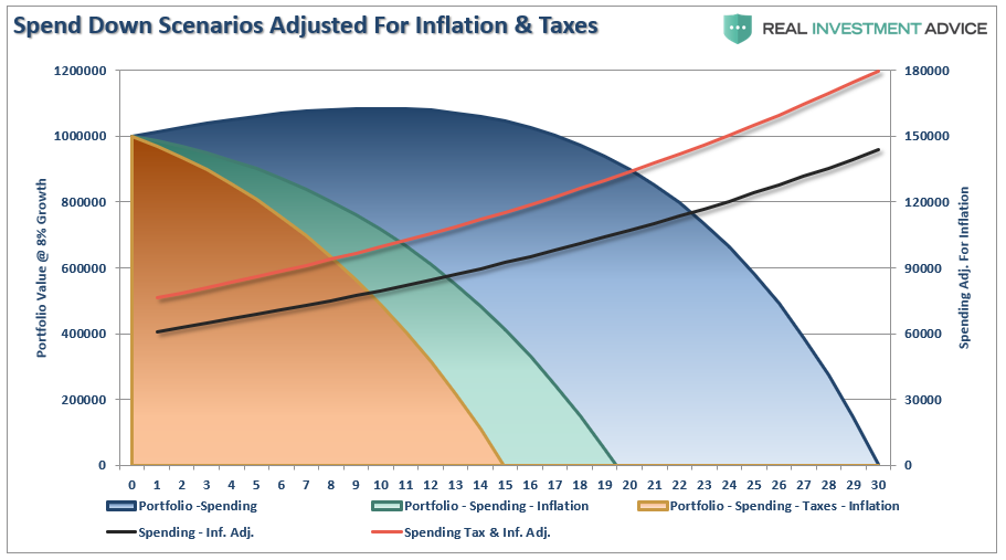
Let’s start with our $1 million retirement portfolio. The chart below shows various “spend down” assumptions of a $1 million retirement portfolio adjusted for an 8% annualized return, the impact of inflation at 3%, and the effect of taxation on withdrawals.

By adjusting the annualized rate of return for the impact of inflation and taxes, the life expectancy of a portfolio grows considerably shorter. Unfortunately, this is what “really happens” to investors over time, but is never discussed in mainstream analysis.

To understand “real outcomes,” we must adjust for variable rates of returns. There is a significant difference between 8% annualized rates of return and 8% real rates of return. 

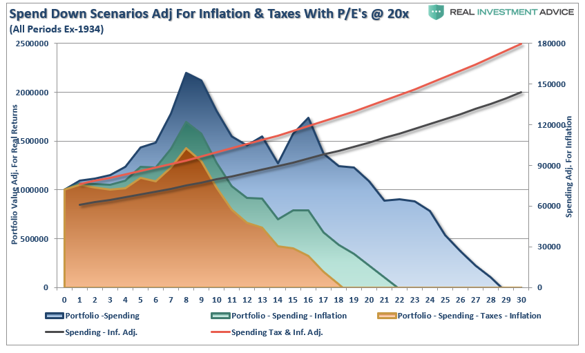
When we adjust the spend down structure for elevated starting valuation levels, and include inflation and taxes, a far different, and less favorable, outcome emerges. Retirees will run out of money not in year 30, but in year 18.

With this understanding, let’s revisit what happens to “buy and hold” investors over time. The chart below shows $3000 invested annually into the S&P 500 inflation-adjusted, total return index at 10% compounded annually, and both 10x and 20x valuation starting levels. I have also shown $3000 saved annually and “stuffed in a mattress.”

The red line is 10% compounded annually. While you don’t get compounded returns, it is there for comparative purposes to the real returns received over the 30-year investment horizon starting at 10x and 20x valuation levels. The shortfall between the promised 10% annual rates of return and actual returns are shown in the two shaded areas. In other words, if you are banking on some advisor’s promise of 10% annual returns for retirement, you aren’t going to make it.

Questions Retirees Need To Ask About Plans

What this analysis reveals is that “retirees” SHOULD be worried about bear markets. 

Taking the correct view of your portfolio, and the risks being undertaken is critical when entering the retirement and distribution phase of the portfolio life cycle.

Most importantly, when building and/or reviewing your financial plan, these are the questions you must ask and have concrete answers for:

• What are the expectations for future returns going forward given current valuation levels? 
• Should the withdrawal rates be downwardly adjusted to account for potentially lower future returns? 
• Given a decade long bull market, have adjustments been made for potentially front-loaded negative returns? 
• Has the impact of taxation been carefully considered in the planned withdrawal rate?
• Have future inflation expectations been carefully considered?
• Have drawdowns from portfolios during declining market environments, which accelerates principal bleed, been considered?
• Have plans been made to harbor capital during up years to allow for reduced portfolio withdrawals during adverse market conditions?
• Has the yield chase over the last decade, and low interest rate environment, which has created an extremely risky environment for retirement income planning, been carefully considered?
• What steps should be considered to reduce potential credit and duration risk in bond portfolios?
• Have expectations for compounded annual rates of returns been dismissed in lieu of a plan for variable rates of future returns?

 If the answer is “no” to the majority of these questions. then feel free to contact one of the CFP’s in our office who take all of these issues into account. 

Yes, not only should you worry about bear markets, you should worry about them a lot.

“TIME is the most important factor in determining market movements and by studying the past records of averages or individual stocks you will be able to prove for yourself that history does repeat and that by knowing the past you can tell the future.”  W.D. Gann, 1939

The analysis and forecasts presented in this article are based on the analytical framework of W.D. Gann.  Gann is an investing legend, labeled as genius by many financial historians.  He reportedly accumulated $50 million in profits during his trading career.  His superior track record and those of others using his methods argues that, regardless of our opinion of his methodology, we should heed the advice of his work.

A more detailed explanation of his analytical framework is included in the last section of this article.

Forecast: 2018-2020

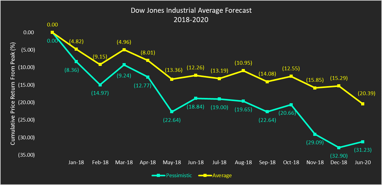
The Dow Jones Industrial Average forecast, in the graph above, is based upon the natural 20-year cycle that Gann identified.  The lines in the graph show the projected monthly cumulative percentage returns from the peak level.  The yellow line is the average scenario and the aqua line is the pessimistic scenario.  The graph provides monthly estimates for 2018.  The last data point represents June 2020, which covers the entire 30-month period from December 2017.

My average scenario forecasts a -15.29% price return for 2018.  The cumulative price return is forecast to bottom in June 2020 at -20.39%, at which time an extended rally should ensue.

My pessimistic scenario forecasts a -32.90% price return for 2018.  The cumulative price return is forecast to be little-changed in June 2020 at -31.23%, at which time an extended rally in should ensue.

20-Year Cycle: Timing Analysis

The New York Stock Exchange (NYSE) began trading operations in 1792.  However, the natural cause of the 20-year cycle first occurred in 1801.  Accordingly, a proper analysis of the 20-year cycle must begin with 1801 as a starting point.  The explanation for this is provided in the section entitled The Natural Cause of the 20-Year Cycle.

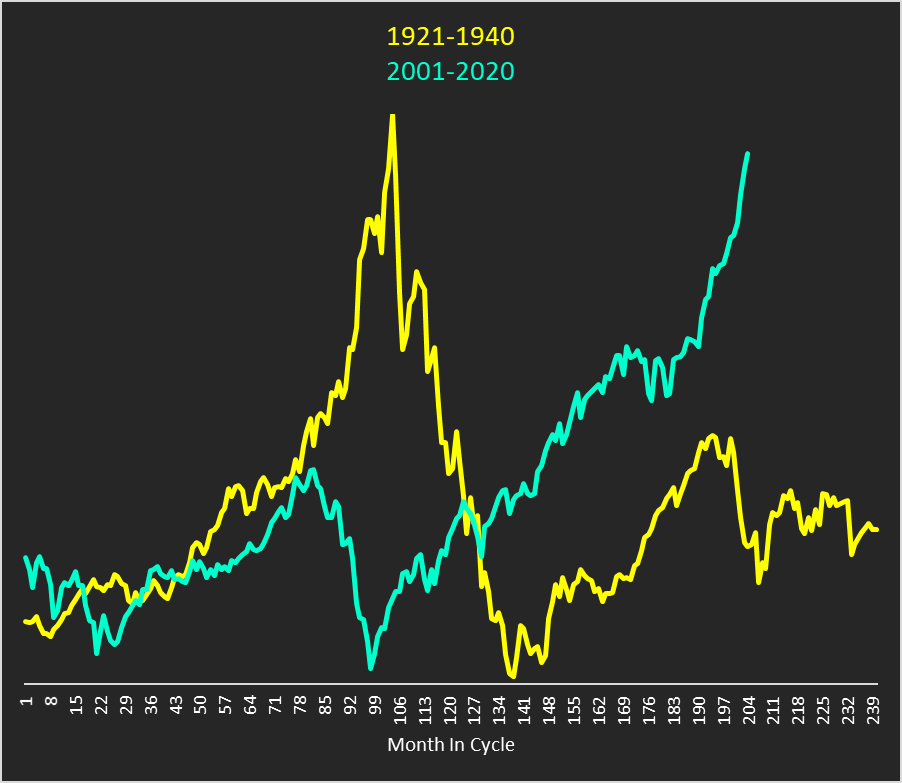
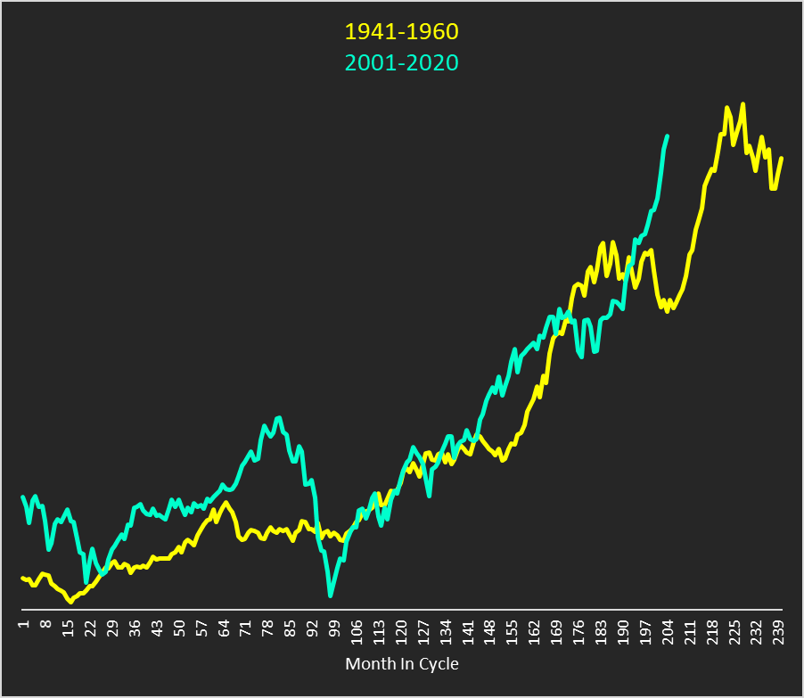
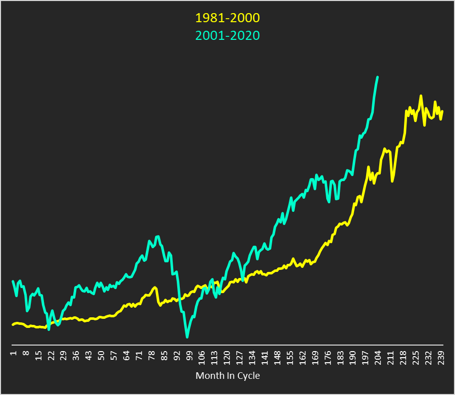
The 20-year cycles, from the inception of the NYSE, consist of the following time periods: 1. 1801-1820, 2. 1821-1840, 3. 1841-1860, 4. 1861-1880, 5. 1881-1900, 6. 1901-1920, 7. 1921-1940, 8. 1941-1960, 9. 1961-1980, 10. 1981-2000, and the current cycle 11, 2001-2020.  Due to limitations of acquiring historical data, the data set of the Dow Jones Average used in this analysis consists of monthly closing prices beginning in January 1901, the sixth 20-year cycle.

To use the data effectively and prepare a forecast, I compare the progression of the current 20-year cycle (2001-2020) with the previous five 20-year cycles, beginning in 1901.  The following five graphs display the comparisons.  Price levels are indexed to 1.00 in month 1 of the cycles and, although not labeled on the graphs, that is the scale of the Y-axis.

As seen in the preceding graphs, the current 20-year cycle has some similarities and some differences with the five previous 20-year cycles.  Based on that visual analysis alone, the individual correlations are not strong enough to base investment decisions on.

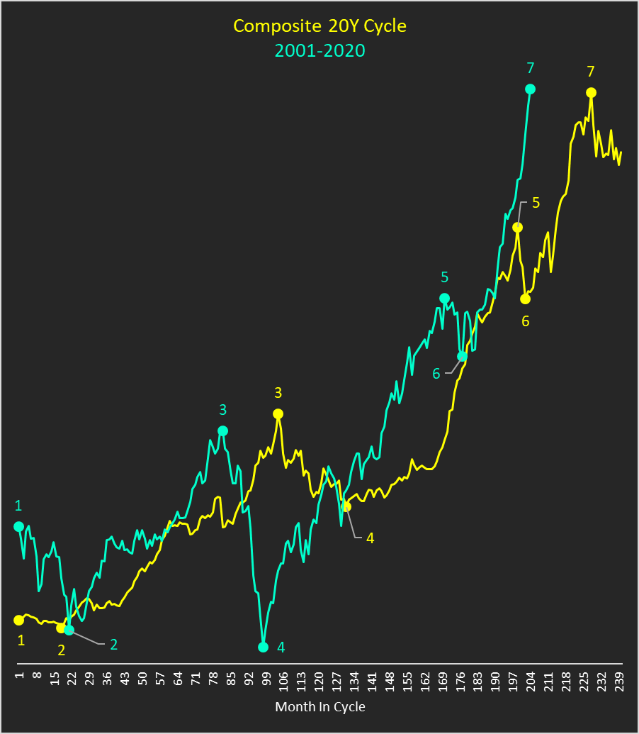
Undeterred by the results from the individual comparisons, I built a composite 20-year cycle.  The components of the composite 20-year cycle are the five historical individual 20-year cycles shown in the preceding graphs.  The composite 20-year cycle averages those five cycles and, importantly, does not include data from the current 20-year cycle.  The following graph displays the composite 20-year cycle overlaid with the current 20-year cycle.  Price levels are indexed to 1.00 in month 1 of the cycles and, although not labeled on the graphs, that is the scale of the Y-axis.  Significant peaks and troughs are labeled as points 1-7 on both cycles.

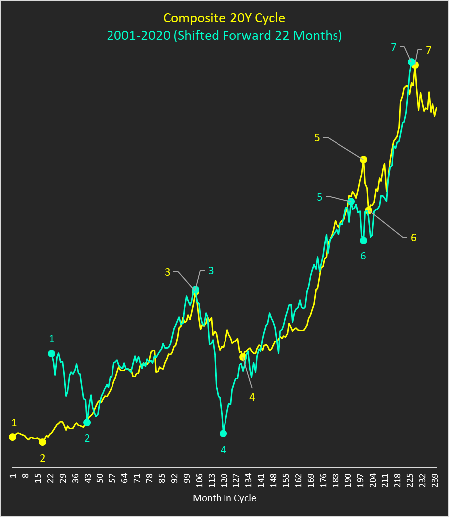
While the correlation of the current 20-year cycle to the composite 20-year cycle is strong, you may have noticed that the current 20-year cycle is progressing faster through peaks and troughs than the composite 20-year cycle.  As a result, I “shift forward” (move to the right) the line of the current 20-year cycle by 22 months.  With the data shifted, the timing of the peaks, troughs, and congestions are virtually identical.  As displayed, the graph and data suggest that December 2017 is the peak of the current 20-year cycle.

20-Year Cycle: Price Return Analysis

The second step in this analysis is to compare the actual price returns for the identified 20-year cycles.  To do so, I identified the seven peaks and troughs within each respective 20-year cycle (points 1-7).  This allows for the comparison of the differences in duration between the pivot points of the composite 20-year cycle and the current 20-year cycle.  The following table maps points 1-7 with the appropriate month in the cycle and with the actual months for individual 20-year cycles:

With the actual dates signifying the composite peak and trough for each historical cycle, I then calculated the percentage price returns between each point in the composite 20-year cycle for each historical cycle.  This allows for comparison of differences in the magnitude of the price moves from point to point.  The following table contains the results.

The final step in this analysis and, the most important in preparing my forecast, is to identify what happened once point 7, the final peak of each 20-year cycle, was reached.  Not only did I look at the following twelve months, but I continued the analysis into the beginning of the ensuing cycle (point 2 of the new 20-year cycle).

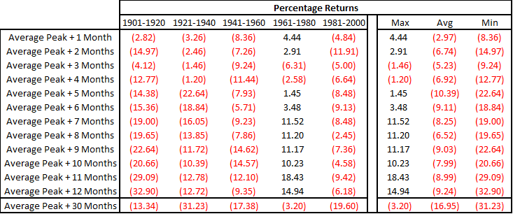
Using the dates identified as point 7 in the preceding tables, I calculated cumulative percentage returns from the peak price level for each 20-year cycle.  For the first year, these are calculated monthly.  The final observation is labeled “Average Peak + 30 Months”, which is point 2 of the following cycle.  Historically, after the low at point 2 is reached a rally begins which is extended in both price and time.  The following table contains the results.

In 4 out of 5 historical 20-year cycles, 80% of the sample, the cumulative percentage returns from the peak price level is negative in every month of the first 12 months following the peak.

In 5 out of 5 historical 20-year cycles, 100% of the sample, the cumulative percentage returns from the peak price level is negative 30 months following the peak.

One historical 20-year cycle, 1961-1980, stands out in the forward-return table due to its positive returns.  The forward returns in this period include the months from January 1980 to June 1982.  Five unique factors contribute to these positive returns:  1. demographic tailwind (the baby boomers were entering their prime earning and spending years), 2. tax-deferred retirement savings accounts were legally created in 1978, 3. mutual funds were relatively new and experiencing tremendous growth, 4. financial deregulation and, 5. consumer credit expansion was beginning in earnest.

To prepare my Dow Jones Industrials forecast, the average scenario uses the average historical experience, excluding the 1961-1980 20-year cycle.  The demographic and legislative factors listed above that bolstered returns in the early 1980’s are now largely turning into headwinds.  Also, I hold the belief that financial deregulation and the resulting financial engineering has reached its zenith.  Additional financial deregulation will have minimal benefits going forward.  Lastly; consumers, state governments, and the federal government have accrued outstanding debt levels so large that make the continued growth of debt increasingly challenging.

My pessimistic scenario uses the minimum percentage returns identified in the preceding table.  Arguably, that may turn out to be conservative as my fundamental valuation model, alone, suggests a -65% decline is warranted.

Scientific & Mathematical Foundation:

Standing on the Shoulders of Genius

In his book How To Make Profits in Commodities, W.D. Gann makes the statement that everything in existence is based on exact proportion and perfect relation.  He also states that, in nature, there is no chance because mathematical principles of the highest order are at the foundation of all things.  “As Faraday said, there is nothing in the universe except mathematical points of force.”

Michael Faraday (1791-1867) was one of the most influential scientists in history.  He discovered the principles underlying electromagnetic induction, diamagnetism, and electrolysis.  Faraday also established that magnetism could affect rays of light and that there was an underlying relationship between the two.  This led him to study the magnetic properties of the Earth’s atmosphere.  Faraday realized that magnetic energy emerges from the Sun and each of the planets in our solar system.  Further, he explained how these planetary magnetic energies interact with one another, directly affecting how much of the Sun’s magnetic energy reaches the Earth’s atmosphere.  He referred to these magnetic energies as “magnetic lines of force”.  These lines are similar to the idea of Pythagoras’ strings.

Pythagoras of Samos (570 BC-495 BC) was a Greek philosopher and mathematician.  He is credited with many mathematical and scientific discoveries including the Pythagorean Theorem, Pythagorean Tuning, the five regular solids, the Theory of Proportions, the Sphericity of the Earth, and the identity of the planet Venus.  He exerted a profound impact on the philosophies of Plato, Aristotle, and, through them, Western philosophy.  Pythagoras believed that the universe was connected by strings.  The strings were connected to the spirit world at the top and to the Earth below.

W.D. Gann studied the works of both Pythagoras and Faraday.  He frequently referred to “natural law” in his writings.  For example, in his 1929 Stock Forecast Gann stated:

“It is natural law.  Action equals reaction in the opposite direction.  We see it in the ebb and flow of the tide and we know from the full bloom of summer follows the dead leaves of winter.”

What Gann was referring to was his belief, based upon the work of Faraday (which was influenced by Pythagoras), that as the planets in our solar system move through their orbits around the sun, the interaction of their magnetic lines of force changes the amount of magnetic energy from the Sun that reaches the Earth’s atmosphere.  These changes affect every naturally occurring event on Earth, including weather, crop growth, and human psychology.  Because of his belief, Gann spent his life researching how the positions of the individual planets and how the angular relationships of the planets relative to one another affected financial markets.  Gann is also well known for his use of his number sequences in the form of squares, circles, and hexagons.  These number sequences follow a defined mathematical relationship to one another.  It is apparent from this discussion that Gann was both a scientist and a mathematician.  He was financially successful in the application of his research, as evidenced by his published books, students of his correspondence courses, and his now famous 1909 interview in Ticker and Investment Digest.  He reportedly accumulated $50 million in profits during his trading career.

The Natural Cause of the 20-Year Cycle

As I stated on page three, the 20-year cycle has a natural cause.  This natural cause is the conjunction of the planets Jupiter and Saturn.  A planetary conjunction occurs when the difference in longitude between to planets is zero degrees.  If you were looking up into the night sky, the Earth, Jupiter, and Saturn would appear to be in a straight line.  The actual amount of time between the conjunction of Jupiter and Saturn varies from slightly under 20 years to slightly over 20 years.  From the list of historical 20-year cycles presented on page three, a conjunction occurred in the first year of the cycle every time.  This explains why I used 1801 as the starting point of the first 20-year cycle.  Using an ephemeris you can identify the location of each planet, and their angular relationships to one another, throughout history and infinitely forward in time.  The next conjunction of Jupiter and Saturn will occur on December 21, 2020, signifying the start of the twelfth 20-year cycle.

Summary

The power of technical analysis is in its ability to reduce multi-dimensional markets into a filtered two-dimensional space of price and time.  Our methodology applies a consistent framework that identifies key measures of trend, distinct levels of support and resistance, and identification of potential trading ranges.  Our methodology can be applied to any security or index, across markets, for which we can attain a reliable price history.  We look forward to bringing you our unique brand of technical analysis and insight to many different markets.  If you are a professional market participant, and are open to discovering more, please connect with us.

We are not asking for a subscription, we are asking you to listen.