Debt allows a consumer (household, business, or government) to pull consumption forward or acquire something today for which they otherwise would have to wait. When the primary objective of fiscal and monetary policy becomes myopically focused on incentivizing consumers to borrow, spend, and pull consumption forward, there will eventually be a painful resolution of the imbalances that such policy creates. The front-loaded benefits of these tactics are radically outweighed by the long-term damage they ultimately cause.

Due to the overwhelming importance that the durability of economic growth has on future asset returns, we take a new approach in this article to drive home a message from our prior article The Death of the Virtuous Cycle. In this article, we use two simple examples to demonstrate how the Virtuous Cycle (VC) and Un-Virtuous Cycle (U-VC) have benefits and costs to society that play out over time.

The Minsky Moment

Before walking you through the examples contrasting the two economic cycles, it is important to put debt into its proper context. Debt can be used productively to benefit the economy in the long term, or it can be used to fulfill materialistic needs and to temporarily stimulate economic growth in the short term. While both uses of debt look the same on a balance sheet, the effect that each has on the borrower and the economy over time is remarkably different.

In the course of his life’s work as an economist, Hyman Minsky focused on the factors that cause financial market fragility and how extreme circumstances eventually resolve themselves. Minsky, who died in 1996, only recently became “famous” as a result of the sub-prime mortgage debacle and ensuing financial crisis in 2008. 

Minsky elaborated on his “stability breeds instability” theory by identifying three types of borrowers and how they evolve to contribute to the accumulation of insolvent debt and inherent instability.

• Hedge borrowers can make interest and principal payments on debt from current cash flows generated from existing investments.
• Speculative borrowers can cover the interest on the debt from the investment cash flows but must regularly refinance, or “roll-over,” the debt as they cannot pay off the principal.
• Ponzi borrowers cannot cover the interest payments or the principal on debt from the investment cash flows, but believe that the appreciation of the investments will be sufficient to refinance outstanding debt obligations when the investment is sold.

Over the past 20 years, investors have been witness to a remarkable sequence of bubbles. The first culminated when an abundance of Ponzi borrowers concentrated their investments in the equity markets and technology stocks in particular. Technology companies, frequently with operating losses, raised capital through stock and debt offerings from investors who believed excessive valuations could expand indefinitely.

The second bubble emerged in housing. Many home buyers acquired houses via mortgages payments they could in no way afford, but believed house prices would rise indefinitely allowing them to service their mortgage obligations via the extraction of equity.

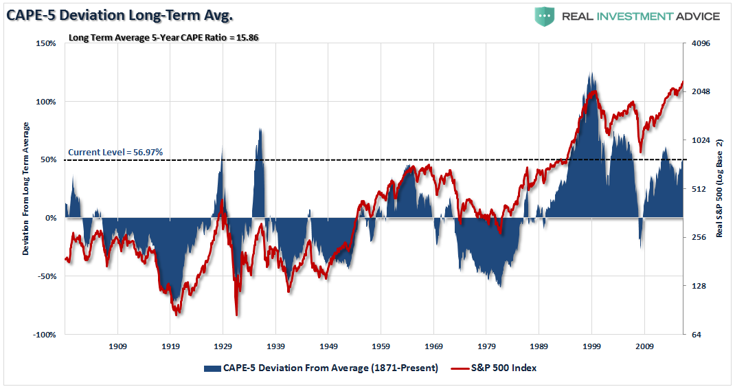
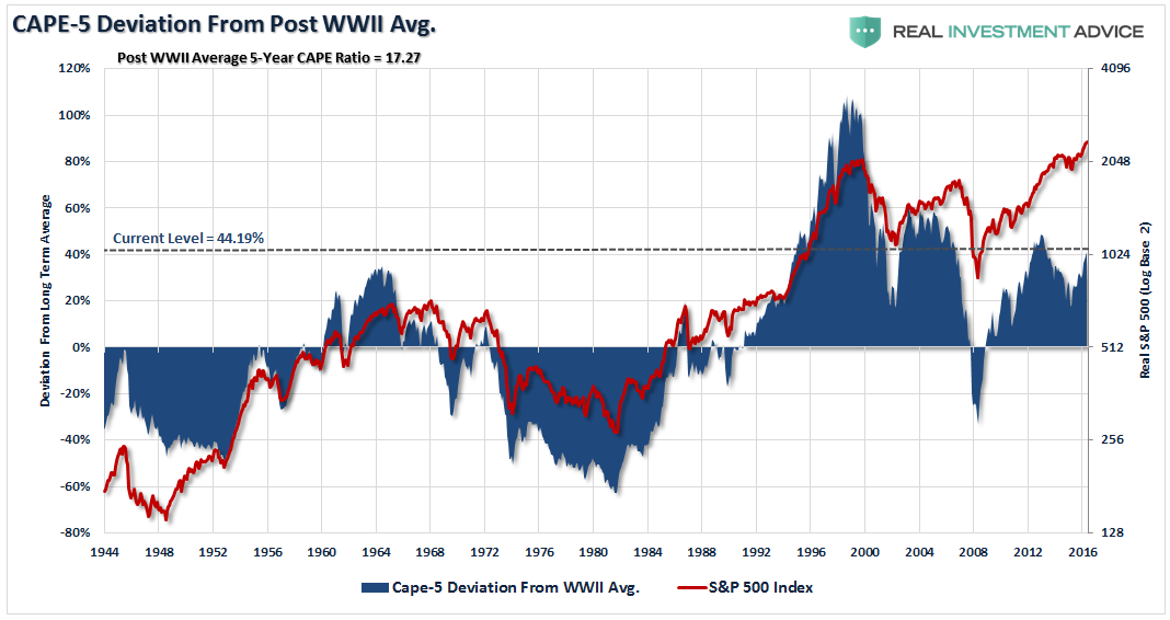
Today, we are witnessing a broader asset price inflation driven by a belief that central banks will engage in extraordinary monetary policy indefinitely to prop up valuations in the hope for the always “just around the corner” wealth effect. Equity markets are near all-time highs and at extreme valuations despite weak economic growth and limited earnings growth. Bond yields are near the lowest levels (highest prices) human civilization has ever seen. Commercial real estate is back at 2007 bubble valuations and real assets such as art, wine, and jewelry are enjoying record-setting bidding at auction houses.

These financial bubbles could not occur in an environment of weak domestic and global economic growth without the migration of debt borrowers from hedge to speculative to Ponzi status.

Compare and Contrast

The tables below summarize two extreme economic models to exhibit how an economy dependent upon “Ponzi” financing compares to one in which savings are prioritized. In both cases, we show how the respective financial decisions influence consumption, profits, and wages.

Table 1, below, is based on the assumption that consumers spend 100% of their wages and borrow an additional amount equivalent to 10% of their income annually for ten years straight. The debt amortizes annually and is therefore retired in full in 20 years.  

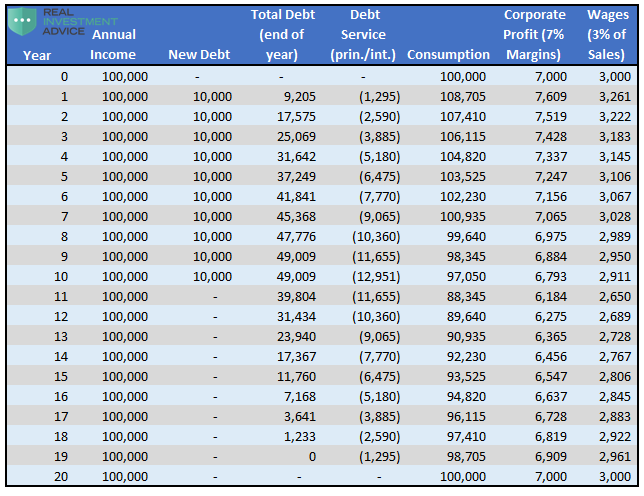
Assumptions: Debt is borrowed each year for the first ten years at a 5% interest rate and ten year term, corporate profits and employee wages are 7% and 3% of consumption respectively, annual income is constant at $100,000 per year. 

Table 2, below, assumes consumers spend 90% of wages, save and invest 10% a year, and do not borrow any money. The table is based on the work of Henry Hazlitt from his book Economics in One Lesson.  

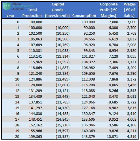
Assumptions: Productivity growth is 2.5% per year, corporate profits and employee wages are 7% and 3% of consumption respectively.

Table 1 is the U-VC and Table 2 is the VC. The tables illustrate that there are immediate economic benefits of borrowing and economic costs of saving. For example, in year one, consumption in Table 1 rises as a result of the new debt ($100,000 to $108,705) and wages and corporate profits follow proportionately. Conversely, table 2 exhibits an initial $10,000 decline in consumption to $90,000, and a similar decline in wages and corporate profits as a result of deferring consumption on 10% of the income that was designated for saving and investing.

After year one, however, the trends begin to reverse. In the U-VC example (Table 1), when new debt is added, debt servicing costs rise, and the marginal benefits of additional debt decline. By year eight, debt service costs ($10,360) are larger than the additional new debt ($10,000). At that point, without lower interest rates or larger borrowings, consumption will fall below the income level.

Conversely, in the VC example (Table 2), savings and investments engender productivity growth, which drives wages, profits, and consumption higher.

The graphs below highlight the consumption and wage trends from both tables.

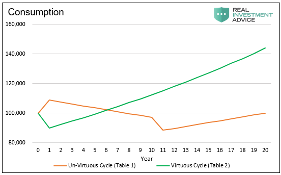
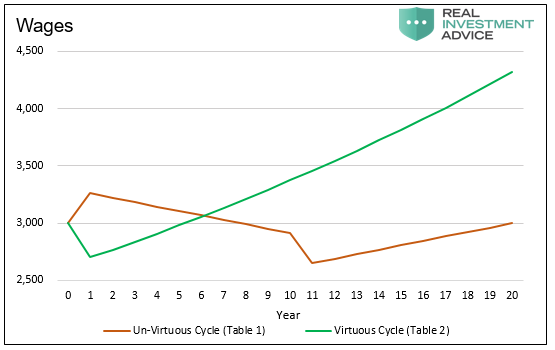
As illustrated in both graphs, the short term justification for promoting the U-VC is prompt economic growth. Equally important, the reason that savings and investments in the VC are admonished is that they require discipline and a period of lesser growth, profits, and wages.

Debt-fueled consumption is an expedient measure to take when economic growth stalls and immediate economic recovery is demanded. While the marginal benefits of such action fade quickly, a longer-term policy that consistently encourages greater levels of debt and lower debt servicing costs can extend the beneficial economic effects for years, fooling many consumers, economists and business leaders into believing these activities are sustainable.

In the tables above, it takes almost seven years before consumption in the VC (Table 2) is greater than in U-VC (Table 1).  However, after that breakeven point, the benefits of a VC become evident as economic growth compounds at an increasing rate, quickly surpassing the stagnating trends occurring under the U-VC.

In the real world, VC or U-VC economies do not exist. Economies tend to exhibit characteristics of both cycles. In the United States, for example, some consumers and corporations are saving, investing, and generating productive economic gains. Productivity gains from years past are still providing benefits as well.  However, over the past 30 years, consumers have increasingly opted to borrow and consume in a Ponzi-like manner and neglect savings. In other words, the U.S. economy has increasingly favored “Ponzi” debt-fueled consumption and denied the benefits of savings and the VC. Then again, U.S. leadership has only encouraged these behavioral patterns through imprudent fiscal and monetary policies.

The U.S. and many other countries are once again approaching what has been deemed the Minsky Moment.  Similar to 2008, this is the point when debt becomes unserviceable and a sharp increase in defaults is unavoidable. Will the Federal Reserve be able to once again reignite “Ponzi” borrowing to suspend that outcome?

Summary

The U.S. and many other countries are forced to deal with the consequences of economic policy actions, borrowing, and consumption behaviors from years past. While the present economic situation is troubling, leadership is obligated to reflect on past choices and move forward with changes that are in the best interest of the country and its entire population. As our title suggests, we can continue to try to pull consumption forward and further harm future growth, or we can save and reward future generations with productivity gains resulting in greater economic growth and prosperity. 

Shifting direction, and “paying forward,” via more savings and investments and the deferral of some consumption, comes with immediate negative consequences to wages, profits, and economic growth. Nothing worth having is easy, as the saying goes. However, over time, the discipline is rewarded, and the economy can be on a more sustainable, prosperous path.

These economic concepts, tables, and graphs extend an accurate diagnosis of the “Death of the Virtuous Cycle.” They are intended to help investment managers better understand the costs and benefits of saving versus borrowing from a macroeconomic perspective. If successful in that endeavor, the substance of this article will afford managers better ideas about how to navigate a very uncertain investment landscape. The implications for the sustainability of economic growth and therefore long term asset returns are profound and the bedrock of all investment decisions. 

In “Part 1” of this series, I discussed at length whether Dr. Robert Shiller’s 10-year cyclically adjusted price-earnings ratio was indeed just “B.S.”  The primary message, of course, was simply:

“Valuation measures are simply just that – a measure of current valuation. If you ‘overpay’ for something today, the future net return will be lower than if you had paid a discount for it.

Valuation models are not, and were never meant to be, ‘market timing indicators.'”

With that said, in this missive I want to address some of the current, and valid, arguments against a long term smoothed price/earnings model:

• Beginning in 2009, FASB Rule 157 was “temporarily” repealed in order to allow banks to “value” illiquid assets, such as real estate or mortgage-backed securities, at levels they felt were more appropriate rather than on the last actual “sale price” of a similar asset. This was done to keep banks solvent at the time as they were being forced to write down billions of dollars of assets on their books. This boosted banks profitability and made earnings appear higher than they may have been otherwise. The ‘repeal” of Rule 157 is still in effect today, and the subsequent “mark-to-myth” accounting rule is still inflating earnings.
• The heavy use of off-balance sheet vehicles to suppress corporate debt and leverage levels and boost earnings is also a relatively new distortion.
• Extensive cost-cutting, productivity enhancements, off-shoring of labor, etc. are all being heavily employed to boost earnings in a relatively weak revenue growth environment. I addressed this issue specifically in this past weekend’s newsletter:

“What has also been stunning is the surge in corporate profitability despite a lack of revenue growth. Since 2009, the reported earnings per share of corporations has increased by a total of 221%. This is the sharpest post-recession rise in reported EPS in history. However, that sharp increase in earnings did not come from revenue which is reported at the top line of the income statement. Revenue from sales of goods and services has only increased by a marginal 28% during the same period.”

• The use of share buybacks improves underlying earnings per share which also distorts long-term valuation metrics. As the WSJ article stated:

“If you believe a recent academic study, one out of five [20%] U.S. finance chiefs have been scrambling to fiddle with their companies’ earnings. 

Not Enron-style, fraudulent fiddles, mind you. More like clever—and legal—exploitations of accounting standards that ‘manage earnings to misrepresent [the company’s] economic performance,’ according to the study’s authors, Ilia Dichev and Shiva Rajgopal of Emory University and John Graham of Duke University. Lightly searing the books rather than cooking them, if you like.”

This should not come as a major surprise as it is a rather “open secret.” Companies manipulate bottom line earnings by utilizing “cookie-jar” reserves, heavy use of accruals, and other accounting instruments to either flatter, or depress, earnings.

“The tricks are well-known: A difficult quarter can be made easier by releasing reserves set aside for a rainy day or recognizing revenues before sales are made, while a good quarter is often the time to hide a big “restructuring charge” that would otherwise stand out like a sore thumb.

What is more surprising though is CFOs’ belief that these practices leave a significant mark on companies’ reported profits and losses. When asked about the magnitude of the earnings misrepresentation, the study’s respondents said it was around 10% of earnings per share.“

As shown, it is not surprising to see that 93% of the respondents pointed to “influence on stock price” and “outside pressure” as the reason for manipulating earnings figures.

• The extensive interventions by Central Banks globally are also contributing to the distortion of markets.

Due to these extensive changes to the financial markets since the turn of the century, I do not completely disagree with the argument that using a 10-year average to smooth earnings volatility may be too long of a period.

Duration Mismatch

Think about it this way. When constructing a portfolio that contains fixed income one of the most important risks to consider is a “duration mismatch.”  For example, let’s assume an individual buys a 20-year bond, but needs the money in 10-years. Since the purpose of owning a bond was capital preservation and income, the duration mismatch leads to a potential loss of capital if interest rates have risen at the time the bond is sold 10-years prior to maturity.

One could reasonably argue, due to the “speed of movement” in the financial markets, a shortening of business cycles, and increased liquidity, there is a “duration mismatch” between Shiller’s 10-year CAPE and the financial markets currently.

The first chart below shows the annual P/E ratio versus the inflation-adjusted (real) S&P 500 index.

Importantly, you will notice that during secular bear market periods (green shaded areas) the overall trend of P/E ratios is declining.  This “valuation compression” is a function of the overall business cycle as “over-valuation” levels are “mean reverted” over time.  You will also notice that market prices are generally “sideways” trending during these periods with increased volatility.

You can also see the vastly increased valuation swings since the turn of the century, which is one of the primary arguments against Dr. Shiller’s 10-Year CAPE ratio.

Introducing The CAPE-5 Ratio

The need to smooth earnings volatility is necessary to get a better understanding of what the underlying trend of valuations actually is. For investor’s periods of “valuation expansion” are where the bulk of the gains in the financial markets have been made over the last 116 years. History shows, that during periods of “valuation compression” returns are much more muted and volatile.

Therefore, in order to compensate for the potential “duration mismatch” of a faster moving market environment, I recalculated the CAPE ratio using a 5-year average as shown in the chart below.

There is a high correlation between the movements of the CAPE-5 and the S&P 500 index. However, you will notice that prior to 1950 the movements of valuations were more coincident with the overall index as price movement was a primary driver of the valuation metric. As earnings growth began to advance much more quickly post-1950, price movement became less of a dominating factor. Therefore, you can see that the CAPE-5 ratio began to lead overall price changes.

A key “warning” for investors, since 1950, has been a decline in the CAPE-5 ratio which has tended to lead price declines in the overall market. The recent decline in the CAPE-5, which was directly related to the collapse and recovery in oil prices, has so far been an outlier event. However, complacency “this time is different,” will likely be misplaced as the corrective trend currently remains intact.

To get a better understanding of where valuations are currently relative to past history, we can look at the deviation between current valuation levels and the long-term average. The importance of deviation is crucial to understand. In order for there to be an “average,” valuations had to be both above and below that “average” over history. These “averages” provide a gravitational pull on valuations over time which is why the further the deviation is away from the “average,” the greater the eventual “mean reversion” will be.

The first chart below is the percentage deviation of the CAPE-5 ratio from its long-term average going back to 1900.

Currently, the 56.97% deviation above the long-term CAPE-5 average of 15.86x earnings puts valuations at levels only witnessed five (5) other times in history. As stated above, while it is hoped “this time will be different,” which were the same words uttered during each of the five previous periods, you can clearly see that the eventual results were much less optimal.

However, as noted, the changes that have occurred Post-WWII in terms of economic prosperity, changes in operational capacity and productivity warrant a look at just the period from 1944-present.

Again, as with the long-term view above, the current deviation is 44.19% above the Post-WWII CAPE-5 average of 17.27x earnings. Such a level of deviation has only been witnessed three times previously over the last 70 years in 1996, 2005 and 2013. Again, as with the long-term view above, the resulting “reversion” was not kind to investors.

Is this a better measure than Shiller’s CAPE-10 ratio?

Maybe, as it adjusts more quickly to a faster moving marketplace. However, I want to reiterate that neither the Shiller’s CAPE-10 ratio or the modified CAPE-5 ratio were ever meant to be “market timing” indicators.

Since valuations determine forward returns, the sole purpose is to denote periods which carry exceptionally high levels of investment risk and resulted in exceptionally poor levels of future returns.

Currently, valuation measures are clearly warning the future market returns are going to be substantially lower than they have been over the past eight years. Therefore, if you are expecting the markets to crank out 10% annualized returns over the next 10 years for you to meet your retirement goals, it is likely that you are going to be very disappointed.

Shiller’s CAPE: Is It Really B.S. – Part 1